


What does success in the game Eurobusiness depend on? From what I remember, when I played this game quite often a dozen years ago, mainly on negotiating talent. If you happen to still play this game, reader, this article may strengthen your negotiating position. We will try to count the probability of players stopping at each field, an important factor affecting the value of the properties they buy. We will use the Monte Carlo method to estimate these probabilities. In the article I will try to show:
- what the Monte Carlo method is and why it is beautiful,
- how to program it in R,
- how to check if the results make sense,
- how to assess whether the number of simulations is sufficient.
First, let's recall what the board for the Eurobusiness game looks like (Figure 1). It consists of 40 fields numbered from 1 (the "Start" field) to 40 ("Vienna"). We have one field that changes position (31, "You go to jail") and six that potentially change position (chance cards: 16 blue and 16 red). We will continue to call them special fields. In addition to this, if the dice throw results in the same number of eyes on both of them, you throw again, moving by as many fields as the total number of eyes that fell in both throws. However, if something like this happens again, we go to jail, that is, to field 11.

How do we count the probabilities of stopping at each field? We can roll the dice and write down where we stood. If we get stubborn and do it really a lot of times, we will get the probability we are looking for by dividing the number of times we stopped on a particular field by the number of all throws. This is the essence of the Monte Carlo method. It's just a matter of making the computer do it instead of throwing the dice itself.
Let's write pseudocode to implement something like this. For simplicity's sake, we'll play with ourselves, since player interactions don't change the position anyway.
1# ustaw się na polu start
2# powtarzaj N razy:
3#   rzuć dwiema kostkami
4#   jeśli liczba oczek nie jest taka sama, przesuń się o sumę oczek
5#   w przeciwnym wypadku rzuć jeszcze raz
6#     jeśli liczba oczek nie jest taka sama, przesuń się o sumę oczek z obu rzutów
7#     w przeciwnym wypadku idziesz do więzienia
8#   jeśli trafiłeś na pole specjalne, zmień pozycje
9#   zapamiętaj, w jakim polu się znalazłeś
Let's start with a simplified version that does not include special fields. Remember that we are going in circles, also field 40 is followed by field 1, not 41 (so we will divide modulo 40). You still have to be careful, because 40 %% 40 = 0, so the position of 0 should be changed to 40. In the following code, we create a 40-element vector filled with zeros, and if we stand on, for example, field 10, we will increase the 10th element of this vector by one. Note, the following code is not written optimally (that is, so that the whole thing executes as quickly as possible), but the emphasis is on readability.
1N <- 1e6 # liczba symulacji
2pola <- numeric(40) # tu zapiszemy, jak często stanęliśmy na danym polu
3pozycja <- 1 # początkowa pozycja (start)
4pola[1] <- 1
5for (i in 1:N) {
6  rzut1 <- sample(1:6, 2, replace = TRUE)
7  if (rzut1[1] != rzut1[2]) {
8    pozycja <- pozycja + sum(rzut1)
9  } else {
10    rzut2 <- sample(1:6, 2, replace = TRUE)
11    if (rzut2[1] != rzut2[2]) {
12      pozycja <- pozycja + sum(rzut1) + sum(rzut2)
13    } else {
14      pozycja <- 11 # idziesz do więzienia
15    }
16  }
17  pozycja <- pozycja %% 40
18  if (pozycja == 0) pozycja <- 40 # uwaga na 40 %% 40
19  pola[pozycja] <- pola[pozycja] + 1
20}
21names(pola) <- 1:40
22barplot(pola / N, col = "cadetblue",
23        las = 1, cex.axis = 0.8, cex.names = 0.8)

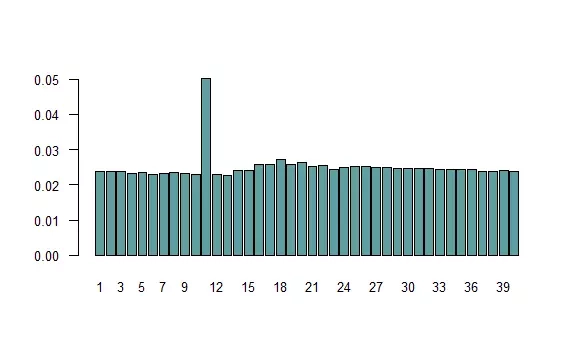
The graph above presents the frequencies of appearance on each field. Let's consider whether they make sense. If repeatedly throwing the same number of eyes would not result in going to jail (box 11), the distribution should be uniform. The probability of such an event is small, so the observed distribution (except for the prison) does indeed resemble a uniform one. Since box 11 is visited more often than the others, hence boxes about 7 meshes away (the most likely sum of two throws) are a bit more popular. Can the fact that the prison is visited about twice as often be explained? Let's calculate. The probability of throwing the same thing on both dice is $$1-over6$$, in which case with a probability of $$1-over36$$ it will happen twice in a row. On the other hand, the probability of standing on any field is $$1over40$$, that is, for a prison of $$1frac{1}{36} + $$1frac{1}{40}$$, so more than twice as much. This is an approximate result, because in giving the value of $$1over4$$, I assumed no jail.
Now let's consider the special fields. We have field 31, from which we always go to jail, in addition to which we take a blue chance card in fields 3, 18 and 34, while in fields 8, 23 and 37 we take a red chance card. Among the blue cards, there are three position-changing cards: "You go back to the start" (1), "You go to prison" (11), "You go to Vienna" (40). Among the red cards, there are seven position-changing cards: "You go back to the start" (1), "You go to Naples" (7), "You go to prison" (11), "You go to Madrid" (15), "You go to Brussels" (24), "You go to the Eastern Railway" (36), "You go back three fields." Thus, we can assume that if we hit a field with a blue card, with probability $$13over16$$ we will not change position, while with probability $$1over16$$ we will move to field 1, 11 or 40. Similarly, in the case of a red card: with probability $$9over16$$ we will not change position, with probability $$1over16$$ we will move to field 1, 7, 11, 15, 24, 36 or go back three fields. Let's write a function that implements the change of position (we will also include modulo division).
1zmien_pozycje <- function(p) {
2  p <- p %% 40
3  if (p == 0) {
4    p <- 40
5  } else if (p == 31) { # idziesz do więzienia
6    p <- 11
7  } else if (p %in% c(3, 18, 34)) { # niebieska karta
8    # z pewnym prawdop. zostań na polu albo zmień pozycje:
9    p <- sample(c(p, 1, 11, 40), 1, prob = c(13/16, 1/16, 1/16, 1/16))
10  } else if (p %in% c(8, 23, 37)) { # czerwona karta
11    p <- sample(c(p, 1, 7, 11, 15, 24, 36, p-3), 1, prob = c(9/16, rep(1/16, 7)))
12  }
13  return(p)
14}
15
16N <- 1e6
17pola <- numeric(40)
18pozycja <- 1
19pola[1] <- 1
20for (i in 1:N) {
21  rzut1 <- sample(1:6, 2, replace = TRUE)
22  if (rzut1[1] != rzut1[2]) {
23    pozycja <- pozycja + sum(rzut1)
24  } else {
25    rzut2 <- sample(1:6, 2, replace = TRUE)
26    if (rzut2[1] != rzut2[2]) {
27      pozycja <- pozycja + sum(rzut1) + sum(rzut2)
28    } else {
29      pozycja <- 11
30    }
31  }
32  pozycja <- zmien_pozycje(pozycja)
33  pola[pozycja] <- pola[pozycja] + 1
34}
35barplot(pola / N, col = "cadetblue", names.arg = 1:40,
36        las = 1, cex.axis = 0.8, cex.names = 0.8)
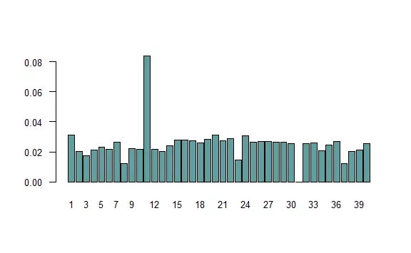
The distribution has changed noticeably. There is a much greater risk of going to jail, with less frequent stops on some fields. This is partly due to the convention adopted: not once do we stop at field 31, as we immediately go to jail. Similarly, fields with a red card are rare, because there is a good chance that we will leave them immediately. However, these fields are of no interest to us, as we cannot buy them.
Someone might reasonably doubt that this whole procedure returns correct results? How can we be sure that what we have obtained are true probabilities? This is due to the so-called Law of Large Numbers. We can look at the individual ratios(fields/N) as the arithmetic mean of $$frac{x1+fields+xN}{N}$$, where $$x_i$$ are equal to 1 when in the $$i$$th move we stopped at a given field, and 0 when we did not. Without going into detail, the Law of Large Numbers says that as $$N$$ increases, such an arithmetic average tends toward the "correct" value (the expected value, in this case the ratio). Someone even more inquisitive, however, might ask whether the observed differences in frequency are not random? Are a million simulations enough? Here, in turn, one can use another, even greater theorem of mathematical statistics, the Central Limit Theorem. We, however, will use a much simpler method: just run the whole thing again (possibly several times). It will turn out that we will get a virtually identical graph, in which case there is no point in increasing the number of simulations.
Finally, let's consider whether these simulations were needed? Since the whole thing depends on the results of throwing the dice and drawing the right cards with known probability, then the problem should be solvable analytically. However, the situation is so complicated that this would be extremely difficult. However, let's imagine that someone brave enough was found. Let's ask ourselves, what is the chance that he did not make at least one mistake? And this brings us to an important reason for using the Monte Carlo method that perhaps not everyone is aware of. Even if an analytical solution is on the horizon, the Monte Carlo method is usually safer, that is, less prone to error. Finally, let's appreciate how simple, and therefore beautiful, this approach is: we simply roll the dice repeatedly and record the results.