Overview and comparison of classification algorithms in Python

Artificial intelligence, including algorithms based on deep neural networks, have become increasingly popular recently. Image generators or complex text-processing models such as GPT are currently in great demand. As a result, many people are thinking about getting the skills needed to train similar models. However, before getting down to training such advanced algorithms, it's worth knowing the basics, i.e. classic machine learning models. They roughly fall into three categories-regression, classification and clustering. Regression is a way of predicting the value of numerical variables-such as price or earnings- based on input data, also in numerical form. Classification also operates on numerical data, but the output of such an algorithm is information in the form of categories, often binary - 0/1, true/false, yes/no. Clustering, for its part, involves detecting so-called clusters in the data, that is, grouping observations based on patterns that have not been previously identified and labeled. Of all these three groups, perhaps the greatest variety of available algorithms is found in the seemingly simplest of the three - classification.

What is classification in the context of machine learning?

Classification is the process of assigning some observation to one of the preconceived categories. An example would be applying for a loan at a bank. Our application can be simplified to a set of numbers such as age, marital status (a categorical variable that can be represented as a number), gender, salary, etc. Then some algorithm, on the basis of these numbers, will have the task of issuing a decision-granting credit (1) or denying it (0). In some problems there may be more than two categories, but binary classification is encountered most often, so these are the problems we will consider. How can such a decision be issued? There are certainly various ways, and one of them is to use the expertise of an expert. An experienced bank employee can assess the risk of default in a particular case and, on this basis, deny the loan. However, despite the high level of knowledge required for such a profession, the decision-making process in this case can be easily automated (and therefore - saved). How? Simply by analyzing the learning data, i.e. a certain number of historical applications (thousands, perhaps even tens or hundreds of thousands) and capturing the relationships that exist between the input data-the characteristics of the applicant-and the decision. This is such a complex problem that it's hard to lay out the right algorithm for a human to analyze the data manually and draw conclusions from it. However, there are ways to automate the decision-making process, and this is where the issue of classification in machine learning comes in.

Examples of classification algorithms

There are different models for classification and each is characterized by different features. Depending on the problem we are working on, we will be able to choose a different algorithm. A few examples are listed below.

Logistic regression

This algorithm is considered one of the simplest and is often not sufficient in complex problems. However, it works well in linear problems, that is, problems where it is always the case that as some input increases, the probability that the result of the classification is class 1 (or 0) increases. For example, if for a group of adult people we want to determine their gender based on height and weight, then by increasing the values of both of these parameters the probability that a person is male always increases. This is because men are statistically taller and heavier. However, if above a certain height limit (e.g., 180 cm) the probability that a person is a woman began to increase, the linear model would prove ineffective.

Here's how logistic regression works. The example below illustrates this for only one input variable "height," but the model can be generalized.

1. We start by putting the predicted category in zero-one form. Ultimately, all processed data must be converted into numbers.
2. Then, for better understanding, let's represent all the learning data on a graph. These are the red points whose position (x, y) results from a combination of parameters (height, gender). Although there is no clear boundary between the height of the two genders, we can see that in women the coordinates along the x-axis are shifted more to the left and in men - to the right.
3. The next key step is to fit a so-called logistic function to the learning data. This function determines the distribution of the probability of belonging to class 1 depending on the value of the trait (that is, the so-called independent variable) and has the form:
   
   where: x- the value of the independent variable, in this example height in [cm] a, b- constant coefficients, the value of which determines the shape of the graph of the logistic function

Fitting this function does not require us to do any calculations, of course, the whole algorithm is implemented in libraries such as sklearn in Python.

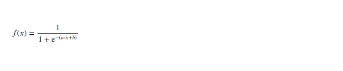
4. Now when we want to determine the gender of a new observation (person) based solely on its height, we need to calculate the value of the logistic function at this point. If this value exceeds 0.5, then we classify the observation as class 1 and otherwise as class 0. Of course, the more features we have at our disposal, the more accurate our model will be-as long as the probability of belonging to each class always increases (or decreases) as the value of the feature changes.

Features of the logistic regression model:

• The model performs quite well in linear problems
• Does not require large amounts of data
• Is unable to capture complex relationships
• Is prone to disturbances caused by outliers in the input data

Decision tree

The decision tree is an algorithm whose primary advantage is the high interpretability of the results. This means that when a trained model assigns a new observation to any of the classes, we are able to explain why that particular decision was made. This is one of the reasons why such an algorithm will work well for the previously presented issue of the decision to grant or deny credit. Such a decision often requires justification and the decision tree provides us with it. The model is based on a series of individual questions that we can answer "yes" or "no" to. By answering them in the right order, we finally arrive at the final decision to which class to assign the observation.

The tree below illustrates a scheme for making credit decisions for applicants who are characterized by characteristics such as:

• Credit history (whether the applicant has a credit history-yes/no)
• Applicant income (applicant's income-numeric variable)
• Coapplicant income (coapplicant income- numeric variable)
• Loan amount (amount borrowed- numeric variable)
• Loan amount term (loan duration in months- numeric variable)

In the first step, we check whether the credit history is 0 (in other words, whether it is <=0.5). If yes (left arrow), we move to the next question about the coapplicant's income. If no (right arrow) then we ask about the duration of credit. Answering further questions, we finally arrive at a node where there are no further questions and the class information on this node (class=0 or class=1) is the result of the classification.

The question may arise- how do we know how to select further questions and the boundary values in them? This is what training the model is all about. Based on the learning data, the questions are selected to best classify the analyzed observations in the least number of them. What follows-we will gradually divide the set of observations into such groups, which to the maximum possible extent will be homogeneous in terms of the occurrence of observations from each class.

Features of the decision tree model:

• Decision trees are highly interpretable
• Their accuracy is quite good even for nonlinear problems
• Trees can be combined into larger ensembles (enseble)
• The model is robust to outliers

K Nearest Neighbors

The last model to be described here is K Nearest Neighbours. This algorithm is very simple and works best for features (input variables) whose dimension is the same, that is, for example, they all specify some size in a particular unit of measurement. It is easiest to understand its operation for data in which there are two features - they will correspond to two spatial dimensions. On such a two-dimensional space, the learning data should be plotted in the form of points. In addition to the position (x, y), each of these points will have information about the class to which it belongs. Then, for each new observation, we check what class the K (any positive integer) nearest neighbors of that point in the given space belong to. We can take the value of K at our discretion, but it is usually less than 10.

(Source: https://www.jcchouinard.com/k-nearest-neighbors/) For example, in the graph above, the green and blue points are learning data belonging to two classes-A and B. We then apply a new observation-an asterisk-to the graph and check to which class most of the K nearest neighbors of the new point belong. In this case, depending on the assumed value of K, the result of the classification will be different.

Features of the K Nearest Neighbors model:

• KNN model is simple to understand and implement
• It works only where the distribution of values for each feature is similar. Otherwise, the data should be rescaled
• The fewer points we choose, the more overtrained the model will be*(overfitting*)

Summary

The models described here are only selected examples of classification algorithms. There are many more, and each has its own characteristics, advantages and disadvantages. Other classifiers you should consider learning about are:

• Support Vector Machines
• Naive Bayes Classifier
• Random Forest Classifier
• Gradient Boosting Classifier

Learning can be helped by the website kaggle.com where we can find not only data on which we will train our models, but also competitions where we will face other data scientists and see how our classifiers will perform in comparison with their algorithms. The Classification Algorithms in Python workshop held regularly at IT Station, which introduces the topic of classification from complete basics, can also be helpful.

If you're interested in the article, we encourage you to check out the Python category training courses. Also check out the entire Python Programmer training track: Python basics, Python intermediate and Python advanced.