


Creativity - this is certainly one of the most desirable skills for a pentester's job. In my opinion, supported by practice, knowledge of Data Science greatly expands the analysis of potential threats or vulnerabilities.
I will try through the coming lines of code to present the possibilities hidden in numbers using machine learning. All in the spirit of solving real-world issues, in a practical way, which also means the details of environment configuration and implementation, in addition to creating models on pure data.
Defining the problem
Collecting the right data is one of the more serious problems of software engineering. This time we will deal with neutral data, which can be easily downloaded from an official source, without the need for permission or license restrictions. It's worth keeping this in mind, because on the one hand the data is there, there is an n-infinite amount of it, but not all of it is easy for us to access. I think we will develop the topic at this year's Testathon 2020 workshop.
Our target is data on NBA players. A simple task in theory, but it turns out that data collection is fraught with interesting pitfalls. The starting place is the official nba.com website, but following in the footsteps of many sports associations, the NBA league, also makes it difficult to access raw, unprocessed data. Of course, the task is doable, but not easy, which is why I've included a link with the data below the article so that you can focus on cleaning and analyzing it, rather than searching for it.
I am inclined to the thesis that in many cases the faster and most effective way is to collect data manually, i.e. downloading it from the website, cleaning it in Excel or Jupyter notepad.
Data sources
Working with data goes significantly beyond finding the right model to pre-clean and prepare the data, the first step should always be to understand how to prepare your local environment.
In our case, this will be two steps:
- Creating a virtual environment (for Python 3.6)
- Installing the necessary packages, namely Pandas and Jupyter
Why a virtual environment?
It is separate and completely independent from the main Python installation. Each project, should contain its own environment, which allows you to install unique packages. Physically, it is a new directory on the disk, which contains a copy of Python, after installation it contains only basic packages, and we do not litter our system and have any number of such environments at our disposal, it all depends on our requirements. The solution with a virtual environment makes it easier to share code and put it in the repo, because instead of a whole folder with all the packages, we will put only one with the required versions. The downside, of course, is the decreasing disk space. A clean installation takes up about 30 MB to start with, and with each new package this number increases.
**What is Jupyter?**We can, in very simplistic terms, describe it as a notebook that allows you to create interactive sheets that can contain executable code, descriptions, tables, charts and much more, used, among other things, to present the results of our work with data. The installation of Jupyter itself requires only the command pip3 install jupyter, followed by jupyter notebook. Of course, it's worth installing in a virtual environment, but we'll keep that in mind.
Pandas library?
One of the most important tools used in Data Science or Analytics work. It has a myriad of methods for loading data, viewing it, and checking for empty values, for example. It's worth learning about Pandas' capabilities, as it's practically a 'must have' in Machine Learning, and I know I'm repeating myself, but we'll be talking about it during the workshop.
An interesting trick to help you deal with the Python virtual environment is to create an alias in the .bashrc or .zshrc file, with this solution the environment will activate automatically. As a rule, you can use:


We start working with data by launching Jupyter, using the familiar jupyter notebook command. It will launch the default browser and display a page, allowing you to view existing notebooks or create new ones.
Then you import the Pandas library installed on your local host, specify the path to the directory with the data and you're done... you can browse.

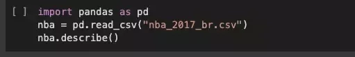

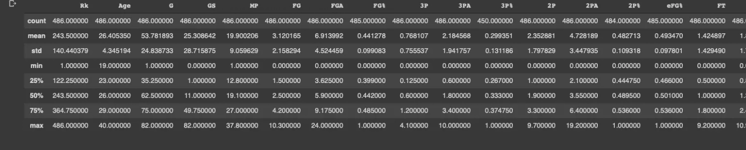
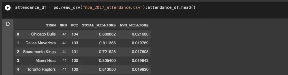
Loading the CSV file itself into the Pandas library, is trivial, as long as the file contains column names and the rows of each are of equal length. In practice, it's never that easy, and it takes an amount of work and time to get the data into the right shape. The describe command from Notebook provides descriptive statistics, including the number of columns and the median for each column. It's worth remembering even at this stage that data analysis requires moving forward continuously, without getting distracted by too much detail, because we can waste a lot of time automating the cleanup of the dataset only to find at the end that all the conclusions from this source were not very helpful.
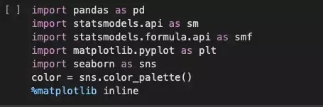
In our data catalog, we have an interesting sheet about teams. It's worth exploring its contents, so we start by importing the necessary libraries.

In the next step, we create a simple Dataset (i.e. collection) for each source.

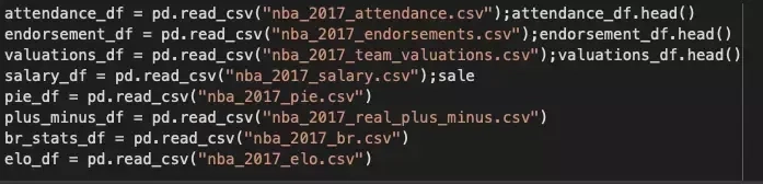
This way we get a chain of Datasets, which is a typical practice when collecting data from distributed sources.

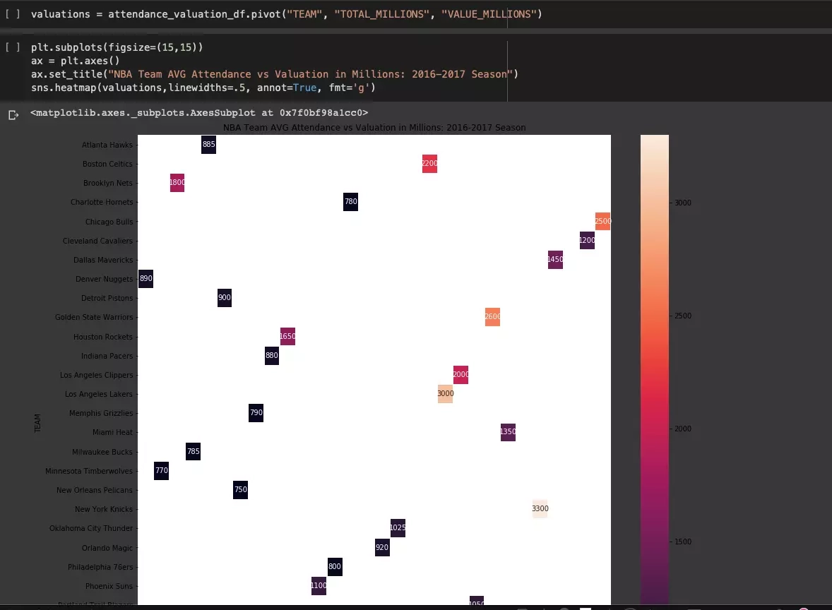
We have the option of combining attendance data with team valuation data:
endorsementdf*= pd.readcsv*("nba2017endorsements.csv");endorsement_df.head()


Using the pairplot function from the Seaborn library, we get a matrix of graphs:

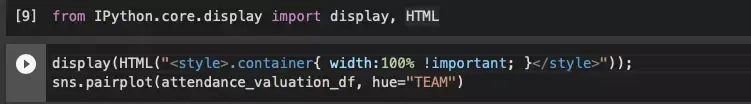


After careful analysis, we can conclude that there is a relationship between attendance and team value, which may not be surprising, but it is worth spending some more time and presenting the relationship using a correlation heatmap:

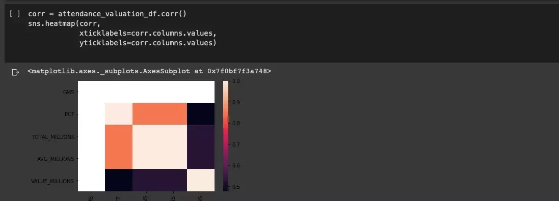
The relationship seen in the graph matrix is even more measurable. We analyze even further using a 3D graph:

Using regression when exploring data
One of the next methods of exploration is the use of linear regression, which is ultimately supposed to make it easier to assess correlations. We will use the StatsModel package, as we want to get a valuable diagnostic output.

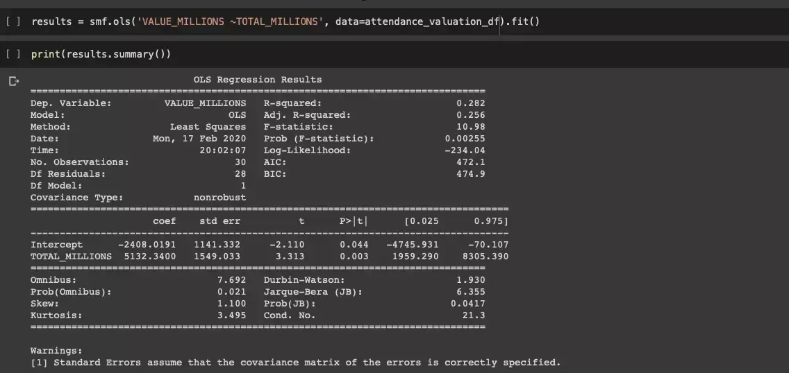
The variable TOTAL_MILLIONS, or total attendance expressed in millions of viewers, is statistically significant in predicting its changes.
Seaborn, which has already been used, includes a built-in and interesting residplot function that allows us to plot the residual for a linear regression:

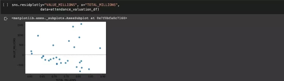
We get confirmation that the pattern was not uniformly random.
Conclusion
There is a relationship between attendance and the valuation of an NBA team, but let's keep in mind the hidden variables, which at this stage only allow us to surmise that factors such as the region's population, average real estate prices (which is taken as a measure of wealth), and how good a team is (percentage of wins) may have an impact
With this set of data, we can turn to more challenging sources. Here we are just getting to know the best and most interesting corners of the work of not only Data Science practitioners, but also pentesters or computer forensic investigators.
Collecting Wikipedia page view data for athletes
We will focus on the following challenges:
- How to extract information about page views in Wikipedia?
- How to find a way to generate links referring to Wikipedia?
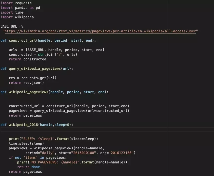
In the code below, we start by showing the URL to the Wikipedia API that allows display pages and modules:
- Requests makes HTTP calls,
- Pandas converts results to Dataframes ,
- Wikipedia detects dependencies between Wikipedia URLs
Thehacker type of code here is not a hindrance, but of course it can be written much better. Sleep set to 0 can prove to be a problem, but only if you run into the limitations of the API used.

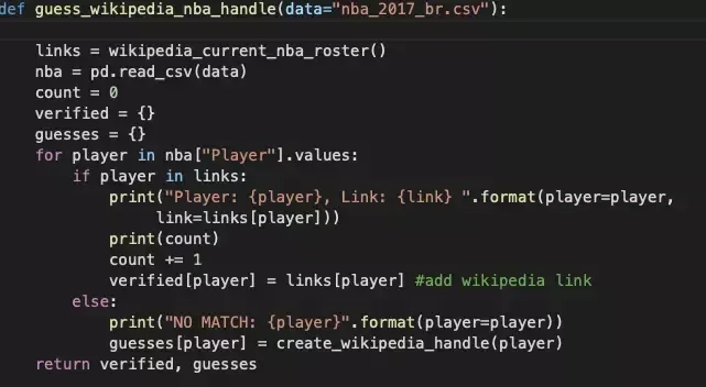
The section of code related to links seems to be more interesting, and for our purposes it takes the form of first_last (it refers to the player's name, of course). It's not likely to be so simple in other examples, but it's worth a try.

Finally, we construct a URL containing a range of data about the athlete.

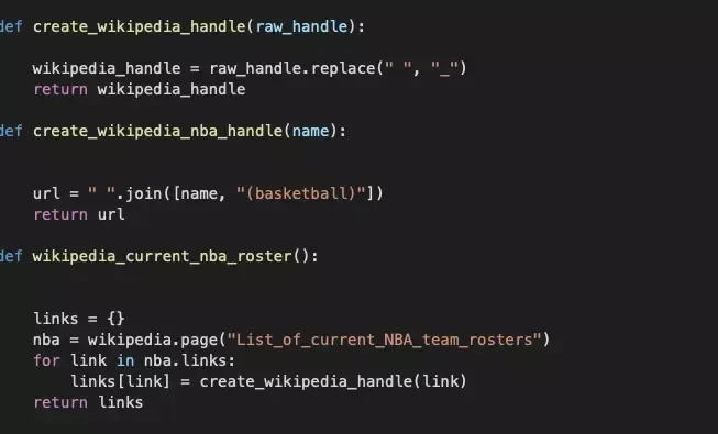
Using the wikipedia library, we can convert the search results for first_last.

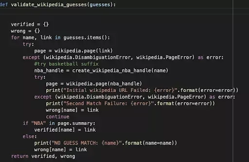
Performing the analysis and, above all, trying to extract the most valuable information for us can take any amount of time :) It all depends on the sources, availability of data, our practice. The above example showed the realism of "fighting" with different data sources, all to solve the originally stated goal.
The example with NBA data was intended to demonstrate that a few quite friendly Python libraries allow a very interesting analysis of any data, looking for interesting dependencies, and thus locating the next sticking points, being a great start for preparing an environment for pentesting or, it is worth noting, helps to assess the importance of the information contained in poorly secured documents, and here it is unnecessary to mention the extraordinary added value in the final report.